Deep Learning with Pytorch-CNN – Getting Started – 2.0

In Deep Learning , we use Convolutional Neural Networks (ConvNets or CNNs) for Image Recognition or Classification. Computer Vision using ConvNets is one of the most exciting fields in current Deep Learning research. For more detail understanding of ConvNets , I will encourage you to go through this amazing Videos tutorials by Andrew Ng

In this tutorial I will try to give you brief intuition about different ConvNets components. From the next tutorial onward we will build a full functioning ConvNets for Image Classification.

Motivation : Why we need ConvNets instead of MLPs?

Large no of Weights to maintain: One of the main drawbacks of MLPs that we need one perception for each inputs , in case of 224*224* 3 RGB image no of weights needs to maintained is more than 1.5 million.

Spatial Correlation is hard to maintain: In case MLPs we need to first flatten the image and then pass it to the MLPs , in this process we can’t keep intact the spatial correlation (example information between two near by pixels)

ConvNets helps us solve this problem using Parameter sharing / Lesser no of parameters to train. First things first – let’s understand few terminologies related to images below –

An image is an matrix of pixel values as shown below –

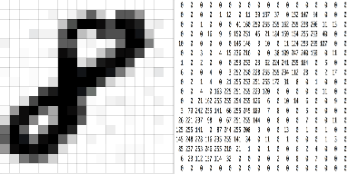
Channel is a conventional term used to refer to a certain component of an image. An image from a standard digital camera will have three channels – red, green and blue – you can imagine those as three 2d-matrices stacked over each other (one for each color), each having pixel values in the range 0 to 255.

Grayscale image, on the other hand, has just one channel. We will have a single 2d matrix representing an image. The value of each pixel in the matrix will range from 0 to 255 – zero indicating black and 255 indicating white.

There are mainly four basic building blocks of ConvNets –

1. Convolution Operator:
ConvNets works on the principle that nearby pixels are more strongly related than distant ones. In Convolution operation we run through a filter (which can have different purposes like detecting edges , eyes , wheels) from top left to bottom right. In Convolution operation the math happens is element wise multiplication then summation.
This operation significantly reduces the number of weights that the neural network must learn compared to an MLP, and also means that when the location of these features changes it does not throw the neural network off.
Filters can also be called ‘kernel’ or ‘feature detector’. Network learns the best value of these filters. Below is an example –

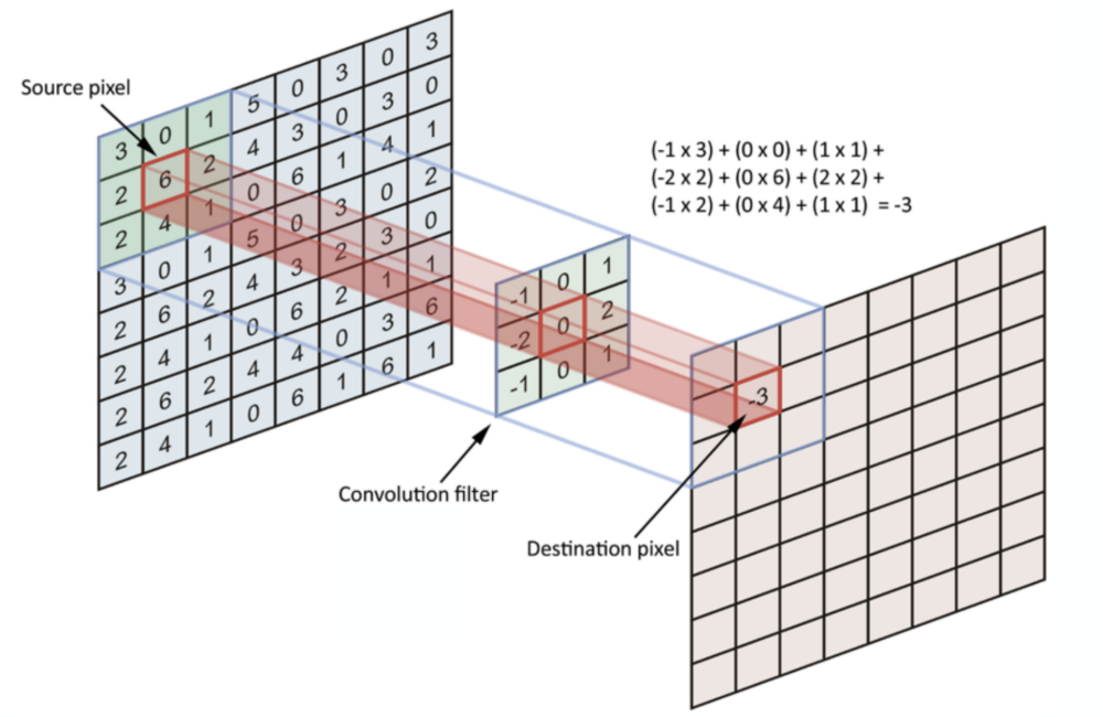
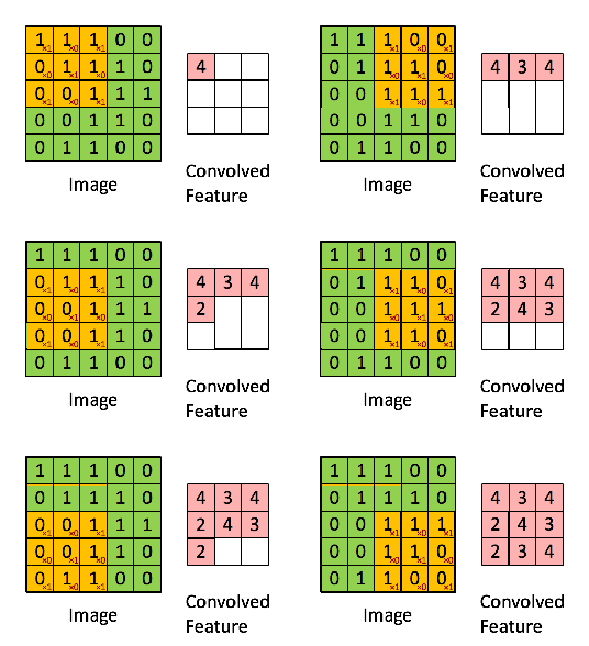
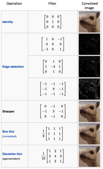
Different values of the filter will detect different features of the images , below are few of the examples –

Strided Convolutions : Suppose we choose a stride of 2. So, while convoluting through the image, we will take two steps – both in the horizontal and vertical directions separately.

2. Padding:
So now if you look closely at the Fig-2 , you will see that edges are only visited once by the filters , though other pixels are visited multiple times , for some of the images this can lead to leaving out the information present at the edges. Introducing zero padding around the edges ensures that information from the edges are also collected during convolution. Below are details of two types of padding –

3. Non Linearity (ReLU):
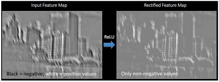
Convolution operation is a linear operation , to introduce non linearity in the network we introduce ReLU. ReLU removes all the negative from the input as shown below. ReLU also tackles vanishing gradient problems.

4.Pooling:
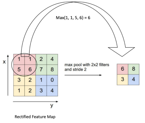
Pooling (also called down sampling) reduces the size of feature map(o/p after convolution operation). By reducing the height and width of the feature map , pooling helps us to reduce over fitting and keeps the dimensions sizes manageable.
There are mainly two types of pooling –
Max Pooling and Average Pooling. Below is an example of average pooling where we run through a 2*2 window and take Max value from that window .In Average pooling instead of taking the max value we take the average value in that windows.

5.Fully Connected Layer:
Output of the pooling is flatted and passed onto to the Fully Connected layer and then to a softmax layer for classification.

Generalized dimensions can be given as:

• Input: n X n X n_c
• Filter: f X f X n_c
• Padding: p
• Stride: s
• Output: [(n+2p-f)/s+1] X [(n+2p-f)/s+1] X n_c’

n_c is the number of channels in the input and filter, while n_c’ is the number of filters.

Some of the popular CNN architecture:

1. LeNet-5
2. AlexNet
3. VGG
4. ResNet

Image Credits/Reference materials:
https://ujjwalkarn.me/2016/08/11/intuitive-explanation-convnets/
https://towardsdatascience.com/simple-introduction-to-convolutional-neural-networks-cdf8d3077bac

Do like , share and comment if you have any questions.