If you have gone through the last three posts of this series , now you should be able able to define the architecture of Deep Neural Network , define and optimize loss , you should also be now aware of few of over-fitting reduction techniques like – compare validation/test set performance with training set , addition of dropout in the architecture.
GPU Support:
Along with the ease of implementation in Pytorch , you also have exclusive GPU (even multiple GPUs) support in Pytorch. In case you a GPU , you need to install the GPU version of Pytorch , get the installation command from this link.
Don’t feel bad if you don’t have a GPU , Google Colab is the life saver in that case. Follow this tutorial to do the set up in Colab.
nn.Sequential:
torch.nn has another handy class we can use to simply our code: Sequential.If you are familiar with Keras , this implementation you will find very similar. Here the modules will be added to it in the order they are passed in the constructor. Choice is yours how you wanna build the NN architecture –
1. By creating a subclass of nn.Module.
2. By creating using nn.Sequential.
We will see a code implementation of this process.
Saving & Loading Models:
Once you train your model and get the desired results , you want to save the model and using this model you would want to make predictions. To provide this facility and to avoid retraining the model every time , we have the functionalities available in Pytorch to save and load model. We will go through the code implementation.
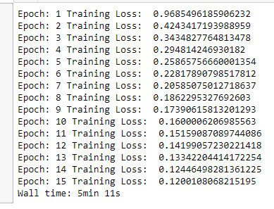
In the notebook we can see that – training the model in GPU – the Wall time: 2min 40s. I have also trained the model in the CPU below are the results.

Do like , share and comment if you have any questions.
