In CNN series , we came to know the limitations of MLPs how it can be solved with CNNs. Here we are getting started with another type of Neural Networks they are RNN(or Recurrent Neural Network).
Some of the tasks that we can achieve with RNNs are given below –
1. Time Series Prediction (Stock Price Prediction)
2. Language Translation/Text Generation.
3. Image Captioning.
4. Sentiment Analysis / Natural Language Processing Tasks.
As you can guess all of these examples maintain a particular sequence. When predicting the output values – you need take in consideration of multiple past values.
Now the obvious question comes why we need another type of NN when we already have NNs (or CNNs). Reasons –
1. MLPs(ANNs) lacks memory.
2. MLPs can’t deal with sequential data.
3. MLPs have a fixed architecture.
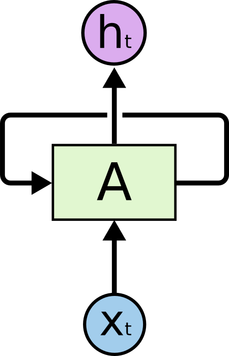
One simple example is stock price prediction. A machine learning algorithm or MLPs can learn to predict the stock price with the given features like opening balance , company revenue etc. While the price of the stock depends on these features, it is also largely dependent on the stock values in the previous days.This can be handled with RNNs typical architecture of RNNs shown below –

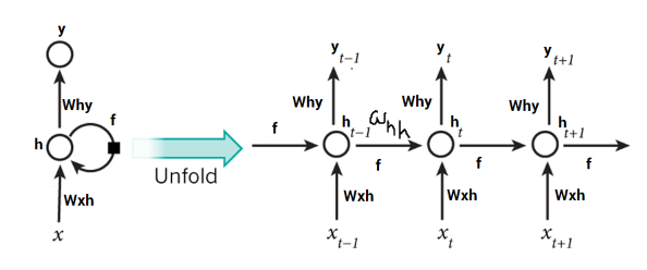
In the above diagram, a neural network, A, looks at some input xt and outputs a value ht. A loop allows information to be passed from one step of the network to the next.Let’s unroll it –

An RNN is multiple copy of the same network that receives inputs at different times as well as it’s previous hidden state.
For example – if the sequence we care about is a sentence of 5 words , the network would be unrolled 5 times , one time for each word.This loop is just the hidden weight getting fed again into the network , but to visualize it , we unroll it to multiple copies of the same network.
Understanding RNN Equations:

Xt is the current state input , weight – Wxh
h(t-1) is previous hidden state output , weight – Whh
Yt is current state output , weight – Why
Current state can be written as –

Once the current state is calculated we can calculate the output –

Back Propagation Through Time:
Once all the time steps are completed the final current state is used to calculate the output yt , The output is then compared to the actual output and the error is generated.The error is then back propagated to the network to update the weights and the network is trained. This is kind of like time traversal – you are going back in the time to change the weights and that’s why we call it back propagation through time.
In case of an RNN, if yt is the actual value ȳt is the predicted value, the error is calculated as a cross entropy loss –
Et(ȳt,yt) = – ȳt log(yt)
E(ȳ,y) = – ∑ ȳt log(yt)
We typically treat the full sequence (word) as one training example, so the total error is just the sum of the errors at each time step (character).So the steps are
- The cross entropy error is first computed using the current output and the actual output.
- The gradient is calculated for each time step with respect to the weight parameter.
- Now that the weight is the same for all the time steps the gradients can be combined together for all time steps.
- The weights are then updated.
Few types of RNN examples are given below –

In the next tutorial we will do a hands on problem solving with RNN in pytorch.
Image/Reference Credits:
https://colah.github.io/posts/2015-08-Understanding-LSTMs/
https://www.analyticsvidhya.com/blog/2017/12/introduction-to-recurrent-neural-networks/
Do like, share and comment if you have any questions.
