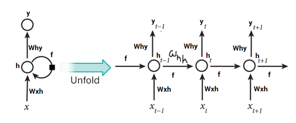
In the previous post of this series , we learnt about the intuition behind RNNs and we also tried to understood how we can use RNNs for sequential data like time series.In this post we will see a hands on implementation of RNNs in Pytorch.
In case of neural networks we feed a vector as predictors , however things are bit different in case of RNNs. Here the input to the model has to be a 3D array. Below are dimensions of this 3D array –
1. Number of samples or Batch Size – total number of training examples or batch size.
2. Sequence Length or Time Steps – RNN by definition is recurrent, it unrolls many times when you use it. It unrolls, in the sequence length dimension, as many times as items in your sequence. For example sequence length can be three if you trying to predict the next hour temperature using last three hours predictors as sequence.
3. Input Size – the usual no of features or predictors in your data.
Below is an example –
x = [ [[32,1383],[41,2928],[39,8823],[20,1252],[15,1532]],
[[35,8272],[32,1383],[41,2928],[39,8823],[20,1252]],
[[37,2738],[35,8272],[32,1383],[41,2928],[39,8823]],
[[34,2845],[37,2738],[35,8272],[32,1383],[41,2928]],
[[32,2345],[34,2845],[37,2738],[35,8272],[32,1383]], ]
Shape of this would be (5,5,2).
Below is an implementation of Multivariate Time Series Air pollution prediction of next hour given the predictor values. The idea and credit of this goes to the awesome blog post of Jason Brownlee
I have just converted his tutorial in Pytorch implementation.This is a dataset that reports on the weather and the level of pollution each hour for five years at the US embassy in Beijing, China. You can get the same dataset from this link as shared in the blog post by Jason Brownlee. Now let’s get our hands dirty.
Press up/down/right/left arrow to browse the below notebook.
Do like , share and comment if you have any questions.

