ML Python Tutorials – 1.0 – Dimension Reduction – PCA

Machine Learning can be divided mainly in two sections –

• Supervised Learning – Where we teach the machines with correct answers or labels. Ex – Regression or Classification.
• Unsupervised Learning – We deal with unlabeled data and we either do Clustering or we go for Dimension Reduction.

In this article we will go through the process/techniques of Dimension Reduction methods. Human begins can generally visualize two to three dimensional data. In real world problems we generally deal with much more than 3 dimensions , to visualize and reduce the dimension of the data (losing minimum information) we generally use Dimension reduction reduction.

For example if our original dataset is having d dimension , then after applying Dimension reduction technique we reduce the dimension to n dimension, where n < d.

Before getting into it , lets go through few required mandatory concepts(assuming you are aware of matrix multiplication) –

• Data-Reprocessing (Feature Scaling): Most of the data we encounter in real world contains units ,assume that we have two measures height and weight and we want to create a third variable which is the sum of height(cms) and weight(kgs) , as the measures are in two different scales , the result will not be proper(will be dominated by one variable). What we need to do is to make these values unit free , so that both the variables are in same scale. To achieve this we first subtract mean and divide by standard deviation. This process is called standardization (or Z-score normalization) so that the features will be rescaled and they’ll have the properties of a standard normal distribution with μ(mean)=0 and σ(sd)=1.

 

 

• Co-Variance Matrix:  Variance is a measurement of the spread in a data set. The variance measures how far each number in the set is far from the mean. This works well in one dimensional dataset but say for D dimensional dataset this does not work. Generally for multidimensional dataset formula is as shown below –

So if we do column standardization then the mean becomes zero.  so now the formula for co-variance formula becomes as shown below – 

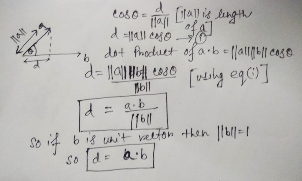
• Projection of one vector to another:
  If we have a vector a and another vector b and the angle between is ϴ. So the project of a onto b is the shadow of a onto b which d.

 

• Eigenvalues , Eigen Vectors: Matrices A (nXn)  has eigenvalues(λ) and eigenvectors(x) if linear operations do not rotate but only stretches the eigenvectors. The eigenvectors remain in the same space or direction post the linear transformation but stretched by corresponding eigenvalues. Matrices A with  eigenvalues(λ) and eigenvectors(x) satisfy the below equation –
  Ax= λx

As the we have gone through the pre-requisites of dimension reduction techniques , lets go through and implement one most popular dimension reduction techniques called PCA.

Principal Component Analysis:

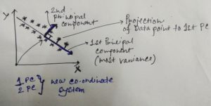
If you have given a dataset of any shape , PCA find a new co-ordinate system from the old co-ordinate system by translation/rotation/projection and it moves center of the old co-ordinate system to the center of the data and it moves first axis (x) to principal axis of the data where the most variation of the data is present and moves the other axis which are orthogonal(perpendicular) to the each principal axis.

As we can see from the above diagram previously we had our regular co-ordinates X , Y. So what PCA will do that it will find – where the maximum variance is present , then PCA will create new co-ordinate system where first PC(principal component) will be assigned with the direction of most variance and other co-ordinates will be orthogonal to the first principal component and so on.Say for this example if we want reduce dimension to one instead of two , PCA will project all the data points to the 1st Principal Component and will ignore second principal component.

Steps of PCA:

1. Compute the mean & Standard deviation of the data matrix and perform standardization.
2. Compute the co-variance of standardize data matrix to help PCA capture the most variance.
3.  Maximum variation of the data lies along the eigenvector of the co-variance matrix corresponding to the maximum eigenvalue. So calculate eigenvector and eigenvalues in pair and do a descending sort on eigenvalues.If we have d dimension in our dataset , we will get λ1,λ2,λ3,…λd (where λ1>λ2>λ3,…>λd). These eigenvalues not only will help us to select eigenvectors(to generate the new orthogonal co-ordinate system) , eigenvalues can also help us to give us way to calculate the % of variance explained with the formula given below.
   
4. Choose the eigenvectors associated with the n (n<d) largest eigenvalues to be the basis of the principal subspace. Collect the eigenvectors in a matrix say B.
5. Do an orthogonal projection of the dataset onto matrix B.

In below notebook we will do step by step implementation of PCA from scratch , along with Scikit implementation.

From the above implementation we can see that with two PCs we can only explain very less variance of the original dataset. So we can go ahead add more PCs to capture more information from original dataset with lesser dimensions.

Limitations of PCA: Does not perform well on the non linear data.

Please leave your questions , comments and feedback below.